Challenges and Advances in Computational Chemistry and Physics, 2011, 409-437
 

Published by Springer

The original publication is available at www.springerlink.com

Volume 13, Linear-Scaling Techniques in Computational Chemistry and Physics: Methods and Applications

Eds.: R. Zalesny, M. G. Papadopoulos, P. G. Mezey, J. Leszczynski

Chapter 15. The Linear Scaling Semiempirical LocalSCF Method and the Variational Finite LMO Approximation

Artur Panczakiewicz, Victor M. Anisimov*

Abstract

When dealing with large biological systems speed determines the utility of the computational method. Therefore in order to bring quantum-mechanical (QM) methods to computational studies of biomolecules it is necessary to significantly reduce their resource requirement. In this light semiempirical QM methods are particularly encouraging because of their modest computational cost combined with potentially high accuracy. However, even semiempirical methods are frequently found to be too demanding for typical biological applications which require extensive conformational sampling. Significant speed up is obtained in the linear scaling LocalSCF method which is based on the variational finite localized molecular orbital (VFL) approximation. The VFL provides an approximate variational solution to the Hartree-Fock-Roothaan equation by seeking the density matrix and energy of the system in the basis of compact molecular orbitals using constrained atomic orbital expansion (CMO). Gradual release of the expansion constraints leads to determination of the theoretically most localized solution under small non-orthogonality of CMOs. Validation tests confirm good agreement of the LocalSCF method with matrix diagonalization results on partial atomic charges, dipole moment, conformational energies, and geometry gradients while the method exhibits low computer memory and CPU time requirements. We observe stable dynamics when using the LocalSCF method.

Keywords

CMO, Linear scaling, LMO, NDDO method, Normalization condition, Orthogonality condition, QM MD, SCF method, VFL approximation

Abbreviations

AM1 – Austin model 1, AO – atomic orbital; B3LYP – Becke 3-term correlation, Lee-Yang-Parr exchange functional; CC – coupled cluster; CI - configuration interaction; CMO – constrained expansion molecular orbital; CPU – central processing unit; DFT – density functional theory; HF/6-31G* - Hartree-Fock method using Pople 6-31G* basis set; HOF – heat of formation; LMO – localized molecular orbital; LocalSCF – local self consistent field; MD – molecular dynamics; MO – molecular orbital; MP2 – second-order Moller-Plesset perturbation theory; NDDO – neglect of differential diatomic overlap; NPT – constant number of particles, pressure, and temperature; NVE – constant number of particles, volume, and energy; NVT – constant number of particles, volume and temperature; PBC – periodic boundary condition; PM3 – parametric method 3; PM5 – parametric method 5; QM – quantum mechanics; RAM – random access memory; SBP – spherical boundary potential; SCF – self-consistent field; VFL – variational finite localized molecular orbital approximation.

15.1 Introduction

Application of quantum-mechanical (QM) methods to biological problems is a long standing goal in simulation science. Solving this problem would bring multiple advancements to computational biology including the expansion of the range of biological applications to bond breaking and formation processes and the increase in general physical accuracy. The more advanced physical model of the QM methods provides a necessary precondition for that.

Significant progress has been made in reducing the computational cost of various QM methods due to the development of linear scaling algorithms.[1,2] However the obtained performance is still insufficient to deal with biological macromolecules. Therefore approximate QM methods are necessary in order to bring QM methodology to the forefront of biomolecular modeling on equal or comparable footing with classical force fields.

In the hierarchy of QM methods semiempirical methods based on neglect of diatomic differential overlap (NDDO) represent the lowest and the fastest level of theory. Their approximate nature and high speed are the two core factors which make them particularly attractive for biological applications. For instance, the chemically accurate hybrid density functional theory (DFT) methods, e.g. B3LYP, have thousand-fold performance overhead over semiempirical methods. This performance bottleneck makes impossible to treat real-size biological systems in presence of explicit solvent. Therefore targeting large molecular systems having inherently dynamic character will require versatile QM methods beyond the performance capabilities of the current ab initio and DFT methods.

Another important aspect of biomolecular simulation is the ability of the selected method to accurately describe condensed phase phenomena. Since all currently accessible non-empirical QM methods (e.g. Hatree-Fock, DFT, and MP2) are not sufficiently accurate for liquid simulations due to missing or insufficient treatment of electron correlation it requires introducing optimized parameters in order to compensate for the deficiency of the level of theory. Semiempirical QM methods provide the necessary solution in the form of their tunable parametric framework. In this regard they are not much different from classical force fields. However being formulated on the quantum-mechanical platform semiempirical methods add an important additional level of physics into the treatment of atomic interactions over the classical mechanics models.

Despite of the computational advantage of the semiempirical theory, it alone is also insufficient to open the door to biological simulations. Since the pioneering work of Karplus and co-workers[3] biological macromolecules have long been recognized as dynamic entities governed by thermal motions. For the latter to be properly accounted one has to use molecular dynamics (MD). This requirement imposes serious performance restrictions on applicability of high levels of theory. Clearly, additional steps beyond replacing matrix diagonalization by linear scaling algorithms are necessary in order to gain additional computational performance. Recognizing this problem prompted the authors to introduce the variational finite localized molecular orbital approximation (VFL).[4,5]

15.2 Theory

15.2.1 Linear scaling problem

According to the quantum-mechanical theory the complete description of the molecular system is included in the wave function of the system, which can be found by solving Schrödinger equation. Since straight forward solution of the Schrödinger equation cannot be made for systems of chemical interest, various levels of approximate solutions are introduced. Historically, Hartree-Fock-Roothan approximation[6-8] provided the first practically useful approach to QM description of molecular systems. In this fundamental method the single-determinant wave function[6] is constructed from 1-electron molecular orbital functions (MO) describing the energy of a single electron in the average field created by all other electrons and nuclei in the system.[6] The MOs are in turn represented by a linear combination of hydrogen-like atomic orbitals (AO) following the Roothaan-Hall approximation.[7,8] Variationally minimizing the linear coefficients of AOs in their MO expansion leads to determination of the molecular wave function.

The Roothaan-Hall approximation to the Hartree-Fock method introduced the important concept of basis set. The type of AOs, their number per atom, and their analytical form are known as basis set. Minimal basis set conceptually originates from hydrogen atom solution of the Schrödinger equation. By analogy, one assigns hydrogen-like 1s, 2s, 2p_x, 2p_y, 2p_z, etc. atomic orbitals to non-hydrogen atoms. Semiempirical methods utilize valence-electron approximation, i.e. including 1s level into a parametric core. This leaves 4 valence AOs 2s, 2p_x, 2p_y and 2p_z as the basis for atoms of the second row. Since the concept of basis primarily serves the numerical purposes of providing variational degrees of freedom more sophisticates basis sets have been introduced such as split-valence bases in which valence AOs are expanded in a linear combination of several functions having independent exponents. Virtually extending the basis splitting process to infinity leads to a complete basis set which provides the Hartree-Fock energy limit. Since Hartree-Fock-Roothaan is a variational method, using a finite basis set provides an upper-bound energy estimation to the theoretical energy limit. Expanding the size of the basis will naturally improve the accuracy of the approximation.

Unfortunately Hartree-Fock method provides incomplete description of electron correlation effects, therefore seeking Hartree-Fock limit is not going to improve sufficiently the quality of the wave function. A solution is provided by DFT, post-Hartree-Fock (MP2, CI, CC), and semiempirical methods. The latter, which are of primary concern in this article, use fitting to experimental data in order to avoid otherwise extremely computationally expensive mathematical operations.

Since semiempirical methods are based on the Hartree-Fock-Roothaan theory they experience similar scalability problems as the Hartree-Fock-Rothaan method yet of obviously lesser severity due to the NDDO approximation. Particularly semiempirical methods scale quadratically in memory storage and cubically in CPU-time with the number of atomic orbitals in the matrix diagonalization step of self-consistent field (SCF) calculations.

Another important part of scalability problem in QM methods is efficient handling of long-range Coulomb interactions. Conventionally in semiempirical methods these calculations scale quadratically in memory storage and CPU time. Since this problem has already been solved in the Fast Multipole Method (FMM)[9] we do not need to worry about this part and instead we will focus on the matrix diagonalization problem only. Several powerful algorithms have recently been developed for the semiempirical framework providing linear scaling alternative to matrix diagonalization.[10-12] The methodological importance of these methods warrants their brief analysis.

It is apparent that the unfavorable scaling of conventional QM methods has the origin in the naturally delocalized character of MOs. Indeed, following the Roothaan-Hall method each MO is expanded over the entire AO-space contributed by all atoms in the system thus leading to full delocalization of MOs over the entire system. To combat the delocalization and the inherent unfavorable scaling of the conventional SCF algorithm one needs to reformulate the Hartree-Fock-Roothaan equations in terms of local interactions.

A remarkable approach is to replace MOs by localized molecular orbitals (LMO) and to seek the final density matrix in terms of LMOs.[10] Since LMOs consume lesser space than delocalized MOs and have fewer variational degrees to optimizes the LMO approach provides valuable memory saving and performance improvement over the use of delocalized MOs when dealing with large systems. This elegant idea is proposed by Stewart and implemented in MOZYME method.[10] In it Jacobi rotations are performed on Fock matrix constructed in the basis of LMOs. The occupied-virtual LMO rotations are carried out to reduce the Fock matrix to block-diagonal form via orthogonalization of occupied to virtual LMOs. Inside the occupied-occupied and virtual-virtual blocks the orthogonalization is not required. During the SCF procedure the LMOs quickly reach the saturation point of about 150 atomic centers and after that they remain roughly constant in size. Since the number of LMOs depends linearly on the number of atoms in the system the method is linear scaling. The small size of LMOs is the determining factor of high performance of the MOZYME method. The main computational overhead in MOZYME comes from slow convergence of the LMO tails.

Another insightful linear scaling approach is presented by the divide-and-conquer method[13] as implemented by Merz and co-workers in semiempirical DivCon program.[11] It utilizes a different powerful resource which can be categorized as a constrained compartmentalization. In this method the entire system is divided on fixed-size compartments which are small enough to be treated via matrix diagonalization. Each part enclosing a group of closely positioned atoms can be viewed as a fixed-size container each carrying their own partial density matrix self-consistently optimized in the electric field created by other compartments. Iteratively walking through the list of compartments one can eventually reach the self-consistency point. The full density matrix of the system is assembled from the compartments density matrices. Because the number of compartments is proportional to the number of atoms in the system the method is linear scaling. The main computational cost in the divide-and-conquer method comes from diagonalization and iterating over the large number of compartments. Increasing the compartment size reduces the iteration cost but increases the cost of diagonalization. Reducing the compartment size reduces diagonalization cost but increases the cost of iterations. Assuming that the compartment size is optimized to maximize the computational performance one obtains the theoretical limit of the method with the diagonalization cost still indirectly controlling the performance of the method.

15.2.2 VFL approximation

Despite of the remarkable improvement in performance of QM methods due to the linear scaling formulations the sheer size of biological macromolecules demands faster computations than the linear scaling of the Hartree-Fock-Roothaan framework can provide. A different strategy is necessary in order to further speed up QM calculations. Such approach was proposed by Anikin et al.[4] by suggesting an additional approximation on the top of the Hartree-Fock-Roothaan method and which is termed variational finite localized molecular orbital (VFL) approximation (Fig. 1).[5]

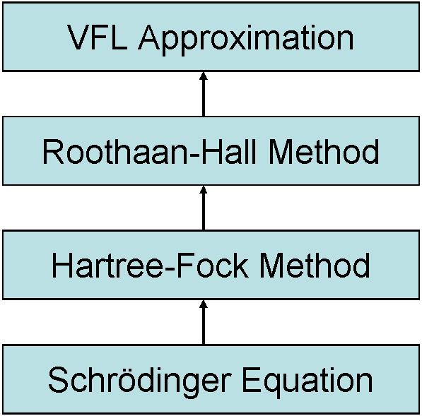
Fig. 1. Hierarchy of QM approximations toward modeling larger systems.

If in the original Roothaan-Hall formulation the density matrix is expressed in the basis of completely delocalized MOs, in contrast to that, the VFL approximation provides a method to compute approximate density matrix in the basis of compact or constrained molecular orbitals (CMO). In VFL the CMO expansion over AOs is fixed and does not change during SCF. Finding the energy and density matrix under the constrained AO expansion is the purpose of the VFL approximation. For example, one may constrain CMO expansion to 5 atomic centers and, based on the VFL approximation, still will be able to variationally determine the density matrix and energy corresponding to such constraint. Obviously, the density matrix constructed under such stringent conditions will deviate significantly from the true density matrix, but important step to realize is the principle availability of such a solution. This opportunity is advantageously utilized in the linear scaling LocalSCF method, which will be discussed in a separate section.

Before starting the derivation of the VFL equations it might be helpful to discuss the concept of CMOs in a greater detail. Since CMOs have limited expansion over AO space they are similar in this aspect to LMOs. However, the distinctive moment of the comparison is that LMO expansion changes during SCF while CMO expansion remains fixed, because it is constrained. The constraint can be trivially implemented by using gradient-based SCF optimization of linear coefficients of CMOs. The non-trivial part is how to maintain orthogonalization and normalization requirements for CMOs.

Normalization counts the number of electrons assigned to MOs. Its numerical value must be unit per MO; any deviation from the unit value will indicate a charge loss or its creation from nowhere leading to computational data making no physical sense. The other determining factor of MOs, the orthogonalization requirement, stems from the concept of independent degrees of freedom like normal vectors i, j, k in the Cartesian coordinate system. If the degrees of freedom are dependent, this is a non-orthogonal case. It is not possible in general to manipulate with dependent variables so the non-orthogonality has to be accounted by employing the inverse overlap matrix.

Orthogonality of MOs can also be obtained via diagonalization but the latter can be applied only when MOs share same AO space, like for example in the divide-and-conquer method. This is not the case of CMOs each having individual AO expansion; hence, diagonalization is entirely inapplicable in the present circumstances. The possible alternative could be to work with non-orthogonal CMOs but such solution is not very appealing because of high computational cost of manipulation with inverse overlap matrix. Therefore we need to find the way to keep CMOs orthogonal at lesser computational expense.

To maintain orthogonality of CMOs during SCF procedure we can utilize a well-known concept of perturbation theory stating that if we know an approximate solution and the expansion series of the target function in vicinity of this point, then there is a mathematically certain way to improve the initial solution. If the non-orthogonality of CMOs is small it can be viewed as a perturbation in the vicinity of the density matrix P(0) = C * C^t constructed from orthogonal CMOs, where C is matrix of linear coefficients of CMOs and C^t its transpose. Next, we can expand the energy of the system, E, into pertubation (Taylor) series around P(0)

     (1)

The unknown final density matrix, P, has the following form considering the general case of non-orthogonality of CMOs

     (2)

where, S is overlap matrix between CMOs. Under the condition that non-orthogonality of CMOs is small the S^-1 matrix can be in turn expanded in Taylor series while neglecting second and higher order terms:

     (3)

where, I is diagonal unit matrix. Combining eq. 2 and 3 one can obtain

     (4)

This provides the opportunity to solve eq. 1. Under the condition of small non-orthogonality we may neglect the second- and higher-order terms in eq. 1 and compensate the missing parts via a penalty term. This produces energy function which approximately maintains orthogonality of CMOs and which is tolerant to small residual non-orthogonality between CMOs:

     (5)

where, W is a penalty matrix, taken for simplicity as a constant.

Now when orthogonality is properly handled the remaining problem is to ascertain normalization of CMOs during the SCF iterations. This is also a non-trivial problem considering that CMOs become interdependent due to the normalization requirement and all CMOs have to be determined simultaneously rather than separately. Conventionally linear coefficients of CMOs can be determined under normalization constraints imposed by the cumbersome method of Lagrange multipliers. Although powerful it is a time consuming procedure. Therefore in order to keep computations at maximum speed we are going to handle the normalization constraints via a computationally efficient approximation. Targeting this goal Anikin et al.[4] suggested an elegant solution to incorporate the normalization constraints into the SCF procedure via variational optimization of generalized degrees of freedom instead of directly manipulating with the linear coefficients of CMOs. These degrees of freedom, R, are formulated in such way to automatically satisfy the normalization condition. It can be shown that when CMO variation δψ_i is orthogonal to the old (before SCF) CMO ψ_i^old the resulting ψ_i^new (after SCF) is automatically normalized at the first order of perturbation theory.

     (6)

     (7)

here φ_μ is atomic orbital.

From      (8)

it follows that      (9)

It means that any variation δψ_i, which is orthogonal to its parent, ψ_i^old, and which minimizes the energy of the system, also preserves the CMO normalization. Correspondingly we can vary coefficients R in order to minimize the energy without the fear of breaking the normalization of CMOs. Optimization of matrix coefficients R can be performed by using a steepest descent gradient minimization procedure.

     (10)

where α is a small constant. Now when ψ_i^new are determined we can deduce linear coefficients of the CMO by using the standard Fourier principle:

     (11)

The equations 5 and 7 summarize the VFL approximation. Since VFL is a variational method the incomplete CMO expansion will lead to upper energy bound according to the theory. Obviously, the larger the expansion the closer the result will be to the conventional Hartree-Fock-Roothaan solution. Molecular properties computed under complete AO expansion would be entirely equivalent to those obtained using canonical MOs. In analogy with the Roothaan-Hall approximation in ab initio methods, which leaves the choice of basis set to the user, the VFL approximation applies no restrictions on the choice of CMO expansion and we are free to choose any non-redundant expansion that suits the task. Once we are concerned with determining the smallest CMO expansion while getting the energy and density matrix as close as possible to the conventional matrix diagonalization we enter the territory of the linear scaling LocalSCF method.

15.2.3 LocalSCF method

The LocalSCF approach to finding the localized solution to the Hartree-Fock-Roothaan method is based on perturbation expansion of the system energy in vicinity of the known approximate density matrix as expressed by eq. 1. Pertaining to LocalSCF, the approximate density matrix, P(0), is the result of the VFL SCF computation. Despite the parallels in utilization of the perturbation theory between LocalSCF method and VFL approximation there are important differences to underline. The VFL approximation is concerned with determining density matrix of the system under the constrained expansion of CMOs. In turn the LocalSCF method uses the perturbation theory in order to gradually lift the expansion constraints aiming to reach the true density matrix of the system while preserving the maximum possible number of the CMO constrains.

The LocalSCF solution to the density matrix is sought iteratively. Having P(0) as a starting point we can get improved density matrix P(1), which we can substitute instead of P(0) and then seek P(2), and so on, each time coming closer to the true Hartree-Fock-Roothaan density matrix, P. This process logically connects the path from density matrix P(0) to P determined on different expansion spaces. The expansion procedure assures the energy convergence under the gradual release of the CMO expansion constraints.

Since the optimal expansion of CMOs is to be determined in the LocalSCF method, one can initiate computations from an initial guess of 2- and 1-center CMOs corresponding to covalent bonds and lone-pairs of the molecular system under study. The VFL SCF procedure can refine the linear coefficients of these CMOs thus producing the density matrix P(0). Now we need to improve this density matrix by choosing the better CMO expansion. This step is the essence of the LocalSCF method.

Having the density matrix P(0) fully relaxed incorporates in it all the information necessary to determine the best possible expansion for individual CMOs, which P(0) is constructed from. LocalSCF identifies the best expansions based on energy criterion, which is estimated according to the first-order perturbation correction

     (12)

where E(0) is energy of the system before expansion, E is estimated energy after expansion of CMO i on AO μ, and R_iμ is the generalized variational degree of freedom of the considered AO.[5]

On the technical side the computer program first creates the list of adjacent AOs for each CMO according to the distance criterion to the already present atomic centers in the CMO. This list represents potential directions for expansion. Then each new AO in the list is tested on the possible energy gain using eq. 12 and only those AOs are retained which produce the energy improvement greater than a threshold value. Such test is performed for each CMO independently. Then the selected AOs having zeroed linear coefficients are added to the corresponding CMOs. Next the expanded CMOs are subjected to the VFL SCF procedure to relax the energy of the system and to determine new density matrix. The CMO expansion and VFL SCF steps are repeated until the energy of the system is converged. If the expansions are not rushed and performed one AO at a time and immediately followed by VFL SCF relaxation of linear coefficients the resulting density function will closely approach the true Hartree-Fock-Roothaan density matrix of the system while constructed from the CMOs having the theoretically possible smallest AO expansion.

According to validation tests[14] the energy of the system in LocalSCF method converges when CMOs acquire about 30 atomic centers on average. Obviously CMOs in LocalSCF all have different sizes because the expansion decision depends on the local environment of each CMO. At this point atomic partial charges, dipole moment, conformational energies, and geometry gradients are well converged in comparison with the result of the conventional matrix diagonalization calculation.[14] After LocalSCF CMOs reach the saturation point of 30 atomic centers the method becomes linear scaling.

Now having reviewed the technical aspects of the proposed algorithm we can compare the advantages of the LocalSCF method with the well-known linear scaling techniques formulated in the framework of MO theory. First and the foremost limitation of the conventional linear scaling methods is that they have little control over the localization process. Typically the degree of localization can be controlled by adjusting various cut-offs and thresholds. However this is a dangerous approach potentially leading to uncontrollable numerical errors. This problem is resolved in the LocalSCF method offering full control over the localization process. Instead of adjusting cut-offs the LocalSCF method offers the mechanism of adjustable SCF constraints in the form of tunable CMO expansion. Correspondingly, we can make CMOs shorter or longer and see what effect it produces on the energy and other physical properties of the system. The VFL SCF procedure variationally adjusts the resulting density matrix to the available CMO expansion space thus always finding the best possible density matrix under the given expansion constraint.

In addition to stressing the differences it might be also illuminating to note conceptual similarities between the LocalSCF and other linear scaling methods. For instance, one can draw parallels between LocalSCF CMOs and MOZYME LMOs. They both represent limited expansion over atomic centers. Next, one may see similarities between the CMO expansion constraints and the compartment size constraints employed in the divide-and conquer method. Having these parallels established one may see clearer what kind of conceptual improvement the LocalSCF method actually brings.

As an improvement over the MOZYME the constrained AO-expansion character of CMOs in LocalSCF eliminates the problem of weakly determined LMO tails. The result can immediately be seen in improved stability of SCF convergence in LocalSCF. As an improvement over the divide-and-conquer method the LocalSCF brings the idea of customization of compartment size to the level of individual CMOs. This leads to drastic reduction in the necessary computer memory. Finally one more analogy can be portrayed. The LocalSCF method and the VFL approximation redefine the large-scale molecular problem in terms of controlled AO expansion. This is reminiscent of using different basis sets in ab initio methods. However, this time the extent of MO expansion over atomic centers is itself a variable parameter which explains the notion that VFL is an approximate extension of the Roothaan-Hall method (see Figure 1).

Since LocalSCF is an approximate method, its main strength of using compact CMOs is also its main weakness. According to validation tests[14] LocalSCF underestimates the heat of formation (which is the analog of potential energy in semiempirical methods) by 5-10 kcal/mol per 1000 atoms. No such problem exists in MOZYME which operates with larger LMOs. The conservative expansion procedure of LocalSCF trained to keep CMOs as compact as possible takes too much CPU time to reach the 150-center AO expansion, making such computation impractical. However reaching this goal may not be entirely necessary, because biological simulations are primarily concerned with relative energy differences, which are typically more accurate.

Additional limitation of the LocalSCF method is related to the condition of reaching the state of saturated CMO expansion, i.e. when CMO expansion stabilizes versus adding new AO to the existing expansion and to removing the least contributing AO from the existing expansion. There are two practically important different saturation conditions, one, taking place when dealing with a rigid-geometry system, and the second condition existing when the system is subjected to geometry changes.

When atoms are fixed in space their position uniquely determines the final result of the CMO expansion. The situation of moving atoms brings additional factors influencing the expansion process. This condition is partially present in geometry optimization calculations but it is mostly distinctive in molecular dynamics simulations. The moving atoms find themselves in a constantly changing neighborhood forcing their CMOs to additionally grow in size vs. the rigid geometry calculation. For instance, in liquid simulations (solvent) molecular fragments can travel on substantial distances in space visiting different parts of the macromolecular system at different time moments. The mobile molecular units carry in their CMOs the atomic orbitals of those atomic centers which they visited some time ago along the simulation path but which no longer satisfy the proximity test. This requires periodically inspecting the CMO expansion and deleting those atomic centers which no longer make a sensible energetic contribution to the given CMO.

What we have in the end is the constantly changing expansion space of the CMOs associated with labile molecular fragments. The processes of CMO growth and compactization eventually reach a dynamic equilibrium resulting in the density matrix which cannot be reproduced in a rigid geometry computation started from the same structure snapshot. In this we have a new phenomenon pertaining to molecular dynamics and geometry optimization jobs in LocalSCF calculations which carry a history of CMO expansion/compactization. As a consequence, single-point energy calculation performed on the final structure after geometry optimization is done would report a less favorable energy of the system than the geometry optimization job came up with. To avoid such confusion LocalSCF dumps density matrix to a computer file after each geometry change. Obviously, single-point calculation restarted from the saved density matrix would produce exactly the same energy as the value reported in the geometry optimization job or molecular dynamics step.

Taking into account this important difference it is necessary to avoid a potential mistake in attempting to compare the energy taken from a rigid geometry calculation with the energy obtained from a flexible geometry calculation. The only sensible energy comparison would correspond to “rigid with rigid” and “flexible with flexible” modes. Similarly in MD simulations the snapshot energies have to be all taken either from the MD output or all recomputed for rigid geometry snapshots extracted from the MD trajectory. Alternatively, one may save the density matrix for each trajectory snapshot to ensure the consistency between the sing-point and dynamic calculations.

15.2.4 SCF convergence criteria

In the LocalSCF computer program the SCF calculation otherwise known as single-point calculation is a complex hierarchical procedure (see Fig. 2). It consists of two iterative levels – micro-SCF and macro-SCF. Each of them is controlled by its own set of convergence criteria.

Fig. 2. Schematic representation of SCF calculation in LocalSCF.

15.2.4.1 Micro-SCF iterations

The micro-SCF computations perform gradient optimization of linear coefficients of CMOs using the VFL SCF procedure under constrained CMO expansion. The linear coefficients of CMOs are optimized iteratively. During the micro-SCF iterations the algorithm checks five termination criteria. Unless specifically mentioned it is enough to satisfy any one of the termination criteria in order to finish the micro-SCF iterations.

First termination criterion, dQthr, monitors the maximal change in diagonal elements of the density matrix between iterations. Since in the semiempirical theory the diagonal elements of the density matrix correspond to atomic charges the current termination criterion actually checks the maximal change in atomic charges between the two consecutive iterations. The SCF procedure will stop when the maximal change drops below the value of the parameter dQthr set to 0.0003 electron units by default.

Second termination criterion, gELMax, looks after the maximum component of the derivative of the energy of the system over generalized variational degrees of freedom, R, corresponding to individual LMO coefficients. This condition will be satisfied when the derivative drops bellow gELMax value set to 0.002 eV/Å by default.

     (13)

Third termination criterion, grNorm, watches for the gradient norm to become smaller than the grNorm parameter set to 0.0005 eV/Å by default.

     (14)

Fourth termination criterion, dEStop, will be satisfied when the energy change between two successive micro-iterations drops below the default threshold value of 0.0001 kcal/mol. The purpose of this criterion is to terminate micro-SCF iterations when the energy change becomes negligibly small but gradient tests are still not satisfied.

     (15)

The dQthr and gELMax termination criteria are always on watch regardless of the computation mode. However, the grNorm and dEStop criteria are applied to input geometry only referred to as single-point calculation. Since the gELMax criterion is more difficult to satisfy than the grNorm and dEStop it automatically implies that the calculations involving geometry optimization and molecular dynamics will be executed under tighter SCF convergence criteria, which is necessary in order to ensure sufficient accuracy of geometry gradients.

Fifth micro-SCF convergence criterion, which is hardcoded, fulfills the role of a fault tolerant switch. The micro-SCF iterations will be stopped if the maximal value of the overlap matrix in the basis of molecular orbitals S_{ij (i≠j)} exceeds the value of 0.07. Normally the overlap integrals should be an order of magnitude smaller. If this cannot be satisfied during the micro-SCF iterations their continuation makes no sense. If this happens the program will exit the micro-SCF iterations and seek help in the CMO expansion procedure.

15.2.4.2 Macro-SCF iterations

The VFL SCF procedure and the CMO expansion step jointly define a macro-SCF iteration loop (see Fig. 2). In the begin of the calculation the initial guess CMOs have too short expansion so running the VFL micro-SCF iterations over them can not produce the final density matrix. The CMOs need to be expanded using the LocalSCF algorithm and then again subjected to the VFL micro-SCF iterations in order to refine their linear coefficients. The macro-SCF convergence criteria determine how many such repetitive cycles of VFL SCF and CMO expansion will be necessary.

The outcome of the CMO expansion at the given macro-SCF step depends on the expansion criterion, ThrDer1, which is a threshold parameter for derivative of the energy of the system over the variational parameter R corresponding to a linear coefficient of AO. The CMO expansion on a new atomic center will be accepted when the expansion gradient for that center is greater than 0.04 eV, which is a default value. Choosing smaller value for the ThrDer1 parameter will result in admitting more atomic centers to the CMO thus quickly increasing its size, and hence, the memory requirement and calculation time. On the other hand, a larger ThrDer1 value may equally produce a negative effect of too slowly growing CMOs and too slowly converging density matrix.

Additional parameter controlling the process of CMO expansion is orthogonality criterion, SijCrt. The algorithm tolerates small non-orthogonality between CMOs. This does not deteriorate quality of the computational results but facilitates faster calculations. The non-orthogonality of CMOs is not supposed to exceed the SijCrt value set to 0.001 by default. In case this criterion is exceeded the problematic CMO will be subjected to an additional cycle of expansion which will improve its orthogonality to other CMOs. Requesting a smaller non-orthogonality threshold than the default value improves the density matrix. However, setting too small value for the SijCrt parameter may lead to a negligible improvement in the energy but quickly raising computational demand.

Final decision to stop the macro-SCF iterations depends on comparison of the energy change between two consecutive macro-iterations against dEEStop parameter. The macro-SCF iterations will be continued until the energy change between the CMO expansions drops bellow dEEStop value set to 0.5 kcal/mol by default.

15.2.5 Quantum-mechanical molecular dynamics

Refocusing the target of QM calculations from small molecules to large systems brings additional challenge besides dealing with the increased number of basis functions. Due to their internal flexibility biomolecules possess huge number of local energy minima and, as a result, the detailed knowledge of the electronic structure of a single local minimum provides insufficient information to predict physical properties of the macromolecule. Therefore geometry optimization developed as the major computational approach in quantum chemical studies of small molecules becomes insufficient when dealing with biological macromolecules. This brings an additional performance requirement that in order for the computational framework to be useful it must be fast enough to make feasible the extensive sampling of conformational space of macromolecules so the expected physical properties of the system can be obtained as statistical average along the dynamics trajectory.

A molecular system evolving in time has electronic and nuclear degrees of freedom to account for. In the original Schrödinger equation the movement of all electrons and atomic nuclei in the system is described via single wave function. However considering a significant disparity between the masses of electron and proton with the ratio of 1836 in favor of proton it is reasonable to decouple the motion of electrons and atomic nuclei thus reducing the complexity of the original equation. This is the essence of the Born-Oppenheimer approximation laying the foundation of the modern QM methods.

Based on the Born-Oppenheimer approximation we can assume atomic nuclei in biomolecule moving according to the classical Newton dynamics while modeling the electron density by quantum mechanical wave function adiabatically adjusting to the instantaneous nuclei configuration. This is called SCF dynamics. In contrast to the classical mechanics MD where the potential energy function is also treated at classical level, the QM MD uses QM level of theory to compute potential energy of the system. This brings additional accuracy to the computational model vs classical approach due to the more fundamental description of electrostatic interactions.

In majority of the technical aspects, except the calculation of the potential energy and geometry gradients, QM MD relies on the same mathematical apparatus originally developed for classical force field MD.[15] In it molecular dynamics trajectory is a result of numerical time integration of the Newton equation

     (16)

where F_i is the total force acting on atom i; m_i is atomic mass; and  is acceleration. Force is determined as negative gradient of the energy, E, over atomic coordinate vector, r_i

     (17)

Giving the initially static atoms a kick in the form of randomly oriented velocities initiates the dynamics. After the initial perturbation subsides and the system relaxes from the internal geometric strain it eventually reaches the thermal equilibrium. This marks the begin of the production run when one can start saving the dynamics trajectory for subsequent analysis. From now on the dynamics can run forever in the absence of non-conservative forces assuming that the computer code is free from accumulation of numerical errors.

15.3 Validation

15.3.1 Linear scaling

Scalability of the LocalSCF method was tested on protein structures 1G5A (9896 atoms), 1HZH (20462 atoms), 3E2P (61504 atoms), and 1AON (119574 atoms) downloaded from the protein databank.[16] These particular proteins were selected based on their roughly doubling number of atoms along the series. The largest selected protein contains a representative number of atoms which is quite exceeding the average number of atoms typically targeted by classical force fields. Since the purpose of the test is to demonstrate linear scalability of the LocalSCF method and its actual resource requirement any other set of proteins would work equally well. Our only preference for the test is using real proteins vs. simplistic systems to stay close to the practical conditions.

The downloaded proteins were cleaned up by removing solvent molecules and adding hydrogen atoms. The protonation state of titratable amino acids was determined at physiological pH. Since these are model gas-phase calculations no counter-ions were added to the systems. Single-point LocalSCF[17] calculations (LocalSCF ver 2.0 Rev 2007.08.27 EM64T) were performed under default program settings on Intel Core 2 Duo 3.0GHz, 4GB RAM desktop working under Linux (Ubuntu 9.04) operating system. Long-range Coulomb interactions were treated via FMM method.[18] Plot of CPU time and required memory over number of atoms are presented in Figures 3 and 4 for PM3[19] and PM5[20,21] Hamiltonians.

Fig. 3. LocalSCF scaling of CPU time over number of atoms for PM3 and PM5 Hamiltonians.

Fig. 4. LocalSCF scaling of required memory over number of atoms for PM3 and PM5 Hamiltonians.

These data show remarkable linear scaling capability of LocalSCF both for CPU time and memory. Single-point calculation of the largest considered protein (GroEL-GroES chaperonin complex; PDB id 1AON) required 1.6 GB RAM and took 2 hours and 10 minutes. Thus semiempirical QM calculations of such and even larger biological systems are now readily affordable on desktop computers. The accuracy of the linear scaling algorithm will be discussed in a separate section.

Additional degree of speed up can be obtained via utilization of multiple processing capabilities of the modern computer hardware. To test parallel scalability of LocalSCF program we took GroEL-GroES chaperonin complex. Calculations were performed using AM1[22] Hamiltonian; exchange interactions were neglected beyond 6 Å distance; CMO expansion threshold derivative ThrDer1 was set to 0.05 eV; the maximal gradient component gELMax was set to 0.05 eV. Long-range electrostatics was treated via FMM method using default program settings. Calculations were performed on a symmetric multiprocessor architecture SGI Altix 3700 computer equipped with Intel Itanium2 1.5GHz CPUs and 256GB RAM, running under GNU Linux. Calculation time was measured for 5 cycles of all-atom geometry optimization and the speedup factor as a function of the number of utilized CPUs is presented in Figure 5.

Fig. 5. Scalability of parallel LocalSCF calculation of GroEL-GroES chaperonin complex.

Considering the general complexity of parallelization of quantum-mechanical codes the presented scalability is quite satisfactory. The scalability is almost linear up to 8 processors and shows less efficient CPU utilization when the number of processors reaches 16. After that point adding more processors to the job is likely not going to further speedup the calculation in the present software implementation.

15.3.2 Accuracy of the linear scaling algorithm

The linear scalability of the LocalSCF method is a direct consequence of using CMOs in contrast to the delocalized MOs employed in conventional SCF methods. Although the individual CMOs have different size in terms of their AO expansion, they are significantly shorter than conventional MOs and less extended than MOZYME LMOs. This fact may raise a concern how reliable are the computational results obtained on such short CMOs and from LocalSCF calculations in general?

To study this subject we performed gas-phase AM1 calculations of proinsulin (PDB id 1EFE) protein containing 60 amino acids and representing the system of 1034 atoms. This is a large system for running semiempirical matrix diagonalization calculations but still affordable as fitting into 1 Gb memory limit so calculations on this system by using MOPAC program[20] would not be too difficult. The protonation state of the titratable amino acids was determined at pH=7 and resulted in the total charge of +1 electron units for the protein. The protein consists of 6 positively charged amino acids (ARG, LYS) and 5 negatively charged amino acids (ASP, GLU). The two histidines present in the protein were modeled in neutral state. The original protein structure was designated as conformation A. The conformation B was obtained by rotating sidechain of TYR26 by 30 degrees toward the hydrophobic protein core.

TYR26 is located at the boundary of the hydrophobic core of proinsulin and has sufficient rotational degree of freedom which won’t create unfavorable short contacts to other amino acids due to the applied sidechain rotation. At the same time the proximity of TYR26 to other amino acids will make the conformational change in TYR26 sidechain visible on potential energy profile of the protein. By introducing this small conformational perturbation to TYR26 sidechain we model energetically accessible structural changes which protein samples during the course of molecular dynamics simulation. Now we want to know how well the energy difference between the two protein conformations computed by matrix diagonalization will be reproduced by the linear scaling LocalSCF method and its underlying VFL approximation. The structurally different parts of the overlaid conformations A and B are displayed in Figure 6 with the rest of the systems hidden from the view.

Fig. 6. The structurally different parts of overlaid conformations A and B of proinsulin. The A (native) conformation is shown in gray. The B conformation having TYR26 sidechain rotated by 30 degrees toward protein hydrophobic core is shown in black.

Matrix diagonalization calculations of the two protein conformations were performed by using MOPAC with default settings. Initial attempts to perform MOPAC SCF calculations were unsuccessful due to convergence problems. As our computational practice demonstrates, gas-phase matrix diagonalization calculations of proteins having high content of ionizable amino acids (4ARG, 2LYS, 4GLU, 1ASP) show systematic convergence problems. These problems worsen with increasing number of ionized amino acids and with increasing number of atoms due to insufficient quality of the generic initial guess and because of general instability of ionized state of proteins in gas-phase. Therefore the density matrix computed by the final LocalSCF method was supplied as initial guess to the MOPAC jobs. After that MOPAC jobs converged in 9 SCF iterations. Using final LocalSCF density matrix as initial guess made the MOPAC calculation looking artificially faster than it would be in the normal case when starting from the generic initial guess. Therefore MOPAC calculation time was projected to 50 SCF iterations in order to obtain a more realistic time estimate. Although the number 50 is based on a pure guesswork its value is absolutely unimportant because even for the absolutely artificial case of MOPAC converging in 9 iterations the LocalSCF computation is still faster by factor of 10 than the superficial matrix diagonalization (see Table 1).

LocalSCF calculations were performed in two modes. One was performed with default program settings, as discussed above, and the second one with tight SCF convergence criterion. These calculation modes are denoted in Table 1 with labels def and acc, respectively. In the accurate mode all the SCF parameters except for the diagonal density matrix elements (dQthr) were intentionally set to such small values so these conditions cannot be satisfied. This forcefully limited the VFL SCF micro-iteration convergence to the criterion of dQthr=0.0003 electron units. The number of CMO expansion steps was limited to 5 and the expansion criterion thrDer1 was set to the negligibly small value of 10^-8. In the factual absence of the energy criterion all the possible CMO expansions found by the proximity criterion were accepted. We also tightened the orthogonality criterion to 10^-8 and increased the cut-off for exchange interactions and for the product of Fock matrix with CMOs to 20 Å.

Table 1. Comparison of LocalSCF in default (def) and accurate (acc) modes with matrix diagonalization (MOPAC) on proinsulin conformations A and B using AM1 Hamiltonian.

^aConformation A.

^bE_conf = HOF_A – HOF_B.

^cRoot mean square difference in atomic charges using MOPAC charges as reference.

^dRoot mean square difference in geometry gradients using MOPAC gradients as reference.

^eAverage size of MOs by the number of atomic centers in their AO expansion.

^fMOPAC calculation time is projected to 50 SCF iterations.

For the analysis of accuracy of the LocalSCF method we selected heat of formation (HOF), conformational energy, partial atomic charges, dipole moment, and geometry gradients, with the results summarized in Table 1. As it was mentioned before, LocalSCF in default mode underestimates the absolute value of heat of formation. In this example the heat of formation is underestimated by 11.53 kcal/mol. However, all other properties are reasonably well reproduced in the default calculation mode. The conformational energy, partial atomic charges and dipole moment are in good agreement with the corresponding matrix diagonalization results. Satisfactory agreement is also obtained for geometry gradients with root means square difference of only 0.34 kcal/(mol*Å).

The LocalSCF CMOs in proinsulin, when obtained in default mode comprise 23 atomic centers on average. For comparison the size of delocalized MOs in the matrix diagonalization calculation of proinsulin is 1034 atomic centers. The use of short CMOs in LocalSCF is the primary reason for underestimation of the absolute value of the heat of formation. Since absolute energy values are of limited use in biomolecular calculations and because the relative properties are accurately reproduced, the default settings in LocalSCF represent a reasonable balance of accuracy vs. performance. The most significant advantage of the obtained speedup is making feasible QM MD calculations of large systems, which will be discussed in a separate section.

The LocalSCF method does not preclude the user from accessing the matrix diagonalization energy limit. In the situations when absolute value of heat of vaporization or highly accurate geometry gradients are needed one can resort to somewhat larger CMOs. The computational results corresponding to such (accurate) mode are presented in Table 1. In the accurate mode the average CMO size grew up to 85 atomic centers. This immediately improved the agreement in the absolute value of heat of formation from 11.53 to 0.55 kcal/mol. Similarly the root mean square difference in geometry gradients dropped from 0.34 to 0.04 kcal/(mol*Å). This is obtained at the cost of 2.7-times slower calculations than the default LocalSCF mode, which is acceptable considering very high performance of the method. The calculation time of the accurate LocalSCF mode is still better by the factor of 46 in comparison to the matrix diagonalization calculation. This is a remarkable speed up considering the fact that the system consisting of 1034 atoms is quite small by biophysical standards. Since the LocalSCF method is linear scaling the level of speed up will be even more impressive when going to real-size biological systems encountering tens of thousands of atoms.

The performed validations tests using just two protein conformations do not sufficiently represent the conformational energy profile of the protein. Although running LocalSCF calculations over an extensive set of protein snapshots is a trivial matter, there are obvious technical difficulties in collecting the reference data using matrix diagonalization due to high computational cost of such calculations. As a compromise, we performed a validation test on 20 proinsulin conformations.[14]

In contrast to the use of a completely dry protein as in the above calculations the new computations included 100 water molecules placed in vicinity of the ionized residues of the proinsulin. This greatly improved stability of the QM calculations. Indeed, zwitter-ionic forms of amino acids are unstable in gas-phase resulting in artificially high polarization making meaningless such QM calculations. Attempts to relax such structure by means of QM calculation produce a number of computational artifacts e.g. disruption of covalent bonds due to hydrogen atom abstraction by anionic centers. Our extensive applications of QM methods to biological systems suggest that proteins in gas-phase cannot have same ionization state as they have in water. This is not a limitation of the QM methods but rather a valuable lesson to comprehend the limits of the classical mechanical models where the notion of protein ionization state originally came from.

According to the performed calculations on the 20 proinsulin snapshots, AM1 and PM3 conformational energy differences were 0.41 and 0.29 kcal/mol, respectively.[14] Dipole moment differences were within 0.1 Debye in both cases. The RMS difference on partial atomic charges was about 0.0003 electron units. The obtained better agreement with the matrix diagonalization data in comparison to our previous tests should be attributed to the water solvation of ionized protein sites and to the use of slightly better SCF convergence criteria.

Now when the general performance and accuracy of the LocalSCF method have been sufficiently established on the relatively small system consisting of a thousand of atoms we may consider performing validation tests on much larger systems. Since in typical biomolecular simulation the simulation box often consists of tens of thousands of atoms we need to prepare a comparable system by the number of atoms. For that purpose we placed proinsulin in a water box with the box walls extending on at least 10 Å in each direction from the nearest protein atom. The system was neutralized by adding a chloride counterion. 20 snapshots of this system consisting of 20,058 atoms were generated using classical force field MD.[14] Since running matrix diagonalization on such large system is beyond the reach of the readily available computer hardware, the reference data were obtained by running LocalSCF calculation while treating all Coulomb integrals explicitly. Since such calculation scales quadratically with the number of atoms it cannot be used when massive calculations are necessary. However, high accuracy of this computation mode and relatively low computational demand make it suitable to generate the reference data to test the quality of the faster LocalSCF calculation modes.

For large systems the LocalSCF program includes the capability to treat long-range Coulomb interactions via the linear scaling FMM method. For the system of 20,058 atoms the FMM provides 9-fold speed up when using AM1 Hamiltonian. Total memory requirement is 256 and 283 MB when using AM1 and PM3 Hamiltonians, respectively. Since the modern desktop computers are equipped with gigabytes of memory we still have sufficient room to treat hundreds of thousands of atoms at QM level on a commodity computer using the LocalSCF method.

Following is a brief analysis of the obtained results for the 20,058 atoms’ system. The accuracy of calculation of partial atomic charges still remained high with the root mean square difference of 0.0016 electron units for AM1 and 0.0003 for PM3 Hamiltonian. The difference in dipole moment increased to 1.1 and 0.2 Debye for AM1 and PM3, respectively, with PM3 again showing the better numerical agreement with the reference data. More noticeable differences were accumulated in conformational energy. AM1 showed 5.4 kcal/mol difference while PM3 resulted in 1.9 kcal/mol difference against the reference data. Although reaching a better numerical accuracy in conformational energy would be desirable the obtained values are still quite satisfactory considering that the comparable MOZYME calculations gave 25.5 and 23.8 kcal/mol differences for AM1 and PM3 Hamiltonians, respectively.

Overall, the QM energy calculations of the 20,058 atoms system taking only about one hour of a single processor time make feasible massive exploration of biological problems based on QM principles. This marks a turning point on the front line of biological simulations where for a long time only classical mechanics methods were practically affordable.

15.3.3 Validation of QM molecular dynamics

Making feasible all-atom quantum-mechanical calculations of large molecular systems is an important step toward better understanding the physics of biological macromolecules. The all-QM approach to biological systems is particularly important in the light of recent studies showing significant differences between classical mechanical and QM description of electrostatic interactions.[23] The charge transfer effects, which are omitted in the classical mechanics model, influence the structural dynamics profile of biomolecules and must be taken into account when targeting the accurate picture at atomic resolution. The net amino acid charges determined from QM MD trajectory showed dependence on the particular amino acid environment. This disagrees with the practice of assignment of unified unit charges to amino acids in classical mechanics, based on mean field approximation. Such unification is acceptable when dealing with isotropic bulk liquids where the mean field approximation has a solid theoretical ground but becomes problematic for biomolecules which are highly anisotropic systems. The fixed-charge electrostatic model and the mean field approximation average out important atomistic details uncovering which is the sole purpose of the biomolecular simulations.

The global character of charge transfer also places certain limits on the range of applicability of hybrid QM/MM schemes representing a rapidly growing theoretical approach to biomolecular simulation.[24] To account for charge transfer effects the entire macromolecular system including protein and solvent should be treated at QM level.

The feasibility of treating large systems entirely at QM MD level is an important advantage of the LocalSCF method. Though, it is still largely unexplored area. There is no sufficient information on how large systems can be treated at QM MD level and what length of simulation time can be approached. These questions will be addressed although at limited degree in the present article.

For the purpose of this study we built a spherical water droplet having the radius of 10 Å. This system contained 141 water molecules or 432 atoms. To prevent the water molecules leaving the droplet due to their kinetic energy during the dynamics run we added a half-shoulder harmonic spherical boundary potential (SBP) with force constant of 10 kcal/(mol*Å). The SBP potential has zero value inside the sphere of the radius of 10 Å while it gently pushes back the water molecules attempting to cross the spherical boundary. The potential acts on non-hydrogen atoms only, hence it does not interfere with any rotational degree of freedom of water molecule. The schematic picture of the SBP potential is given in Figure 7.

Using the droplet model to represent water solvation has obvious disadvantages over the use of periodic boundary condition (PBC). However the SBP model is simple to implement and it is computationally more attractive than the PBC model. This is the reason why we selected the SBP model for validation of the following QM MD calculations.

Fig. 7. Schematic representation of the half-shoulder spherical boundary potential. The energy due to the potential is shown by dashed line. It is zero inside the sphere of radius of 10 Å and has harmonic shape outside the droplet walls.

The water droplet can be simulated using various types of dynamics. First in the list is constant volume – constant energy NVE molecular dynamics, generating microcanonical ensemble of configurations. NVE is the simplest form of molecular dynamics, which can be obtained by direct solution of the Newton second law equations separately written for each dynamic particle in the system (eq. 16). It describes a closed system so no mass or heat exchange with the environment is possible. Since the particles are bound by potential forces that keep them sticking together the volume occupied by the system remains constant during the simulation after reaching the equilibrium state. Though, strictly speaking the rigorous definition of volume requires the presence of walls, like in PBC conditions. No mechanism is available in the NVE dynamics to maintain constant temperature of the system.  The NVE Hamiltonian (H) consists of kinetic (K) and potential (U) energy terms each being a function of N particles having coordinates r

     (18)

The microcanonical ensemble generated by NVE dynamics is not consistent with experimental measurements which are typically performed at constant temperature condition. Therefore practically more useful is isochoric-isothermic molecular dynamics, abbreviated as NVT, which keeps temperature fluctuating around the target value, T₀. The most popular scheme to achieve temperature stabilization while generating a canonical ensemble is the Nose-Hoover algorithm[25] which extends the Hamiltonian by adding a virtual degree of freedom, s, associated with thermostat (aka thermostat coordinate), and which is considered as a dynamic variable

     (19)

where Q is a thermostat coupling parameter (aka thermostat mass), k_B is Boltzmann’s constant. In this equation the particle velocities (determining temperature) are scaled by the parameter s at each time step and the degree of coupling of the real particles with the thermostat is determined by the parameter Q.

With the NVT dynamics and uniform velocity rescaling in general it may happen that due to accumulation of numerical errors the thermostat may start redirecting the kinetic energy from high-frequency modes to the rigid-body rotation and translation degrees of freedom of the droplet, which are not coupled to the internal degrees of freedom of the systems. When happened it would break the momentum conservation thus leading to the “flying ice cube” problem.[26] This is a serious problem when attempting hundreds of picoseconds long NVT simulation of a droplet system under SBP boundary condition. To avoid such problem one would need to apply thermostat equations to internal velocities which provide an explicit mechanism to maintain momentum conservation. Working with internal velocities vs. real ones brings additional computational expense. A simpler solution is to resort to Langevin dynamics given by the modified Newton equation

     (20)

where R(t) is an uncorrelated Gaussian distribution with zero-mean, and γ_i time-independent friction parameters. The random collisions of the real atoms with imaginary solvent molecules eliminate the possibility for an unphysical kinetic energy distribution over the degrees of freedom. It also introduces solvent viscosity into the dynamic equations. Langevin dynamics is a popular method of choice when dealing with molecular clusters in the absence of PBC conditions. On the negative side of the Langevin dynamics is its time-irreversible and non-deterministic character but its numerical stability and the simple way to account for the solvent viscosity outweigh the deficiencies.

Correspondingly we performed 1 ns Langevin dynamics of the water droplet under the SBP condition. During the simulation the temperature was maintained at 300K and the friction parameter was set to 10 ps^-1. The dynamics equations were integrated with the timestep of 1 fs. No constraints were applied to bonds involving hydrogen atoms. First 100 ps of the simulation were considered as equilibration while the remainder of the trajectory was saved for analysis. QM simulations were performed using PM5 Hamiltonian. The 1 ns QM MD simulation took 20 days to run on two cores of an Intel Core 2 Duo 3.0 GHz desktop.

The volume of the system was computed based on the sphere radius defined by the most distant oxygen atom from the center of the sphere. During the simulation the volume of the droplet oscillated around the average value of 4955.10 ų. This corresponds to water density of 0.85 g/cm³ which, as we can see, is underestimated by PM5.

Important indicator of stability of the simulation method is conservation of the virial of the system. In the presence of only conservative forces, which is our case, the following relation known as the virial theorem must hold

     (21)

The potential energy of the water droplet, U = U_int + U_ext, has internal and external components

     (22)

where E is the computed QM energy, F_int,i is internal force acting on particle i due to other particles. The external component of the potential energy is created by the SBP potential

 when |r_i| > R₀; otherwise U_ext = 0     (23)

     (24)

where R₀ is the radius of the sphere where the restraining force is initiated; F_ext is external force with the force constant k₀; r_i is atomic coordinate vector. Eq. 23 and 24 assume the origin of the coordinate system being placed at the center of mass of the droplet.

The plot of virial of the system along dynamics trajectory is displayed in Figure 8.

Fig. 8. Conservation of virial during PM5 MD simulation of water droplet.

Trajectory average of the virial gives the value of -0.6 kcal/mol, which is very close to the expected value of zero thus pointing to stable dynamics.

Having defined the volume of the system we can compute internal pressure inside the droplet based on the virial expression[27,28]

     (25)

where ρ is number density of particles; k_B is Boltzmann’s constant; V is volume of the droplet; F_i is total force acting on particle i due to other particles and soft walls. Eq. 25 can be rewritten in terms of kinetic and potential energy of the droplet

     (26)

Averaging over the dynamics trajectory gives the pressure value of 5.7 atm, which is relatively close to the normal pressure of 1 atm. Using a larger system would make the pressure determination more reliable.

Since the SBP boundary condition introduces distinct volume one may use it to derive a true constant temperature-pressure NPT dynamics. Following the standard approach[29] it is possible to consider volume as another dynamic variable and formulate the corresponding dynamic equations. However, exploring this venue goes beyond the limits of the current article.

15.4 Concluding remarks

Linear scaling LocalSCF method provides a valuable alternative to matrix diagonalization when dealing with large molecular systems. It shows about 50-fold speedup over matrix diagonalization already on such small system as 1034 atoms proinsulin. As a result, QM calculations of hundreds of atoms systems can be readily conducted on commodity computers. Validation tests confirm good accuracy of the linear scaling computations on partial atomic charges, dipole moments, conformational energies and geometry gradients.

The most significant value of the linear scaling LocalSCF method is the feasibility of running QM MD of biological systems thus advancing the computational biophysics to step forward beyond the fixed charge approximation. The presented spherical boundary potential is a computationally economical approach for explicit treatment of water in QM biomolecular dynamics. The 1 fs integration time step makes feasible accumulating hundreds of picoseconds or even nanosecond long trajectories on the modern hardware by utilizing parallel processing capabilities.

The performed water dynamics using PM5 Hamiltonian showed the need to further improve the condensed phase properties of water. The accumulated speedup due to the linear scaling LocalSCF method provides the necessary technical means to succeed in such effort and to move on with the development of accurate biologically oriented semiempirical Hamiltonians.

15.5 References

[1] Goedecker S (1999) Linear scaling electronic structure methods. Rev Mod Phys 71:1085-1123.

[2] Goedecker S, Scuseria GE (2003) Linear scaling electronic structure methods in chemistry and physics. Comp Sci Eng 5:14-21.

[3] McCammon JA, Gelin BR, Karplus M (1977) Dynamics of folded proteins. Nature 267:585-590.

[4] Anikin NA, Anisimov VM, Bugaenko VL et al. (2004) LocalSCF method for semiempirical quantum-chemical calculation of ultralarge biomolecules. J Chem Phys 121:1266-1270.

[5] Anisimov VM, Bugaenko VL (2009) QM/QM docking method based on the variational finite localized molecular orbital approximation. J Comp Chem 30:784-798.

[6] Szabo A, Ostlund NS (1996) Modern quantum chemistry. Dover, New York.

[7] Roothaan CCJ (1951) New developments in molecular orbital theory. Rev Mod Phys 23:69-89.

[8] Hall GG (1951) The molecular orbital theory of chemical valency. VIII. A method of calculating ionization potentials. Proc Roy Soc, London A205:541-552.

[9] Greengard LF (1988) The rapid evaluation of potential fields in particle systems. MIT Press, Cambridge, MA.

[10] Stewart JJP (1996) Application of localized molecular orbitals to the solution of semiempirical self-consistent field equations. Int J Quant Chem 58:133-146.

[11] Dixon SL, Merz KM, Jr. (1996) Semiempirical molecular orbital calculations with linear system size scaling. J Chem Phys 104:6643-6649.

[12] Lee T-S, York DM, Yang W (1996) Linear-scaling semiempirical quantum calculations for macromolecules. J Chem Phys 105:2744-2750.

[13] Yang W, Lee T-S (1995) A density-matrix divide-and-conquer approach for electronic structure calculations of large molecules. J Chem Phys 103:5674-5678.

[14] Anisimov VM, Bugaenko VL, Bobrikov VV (2006) Validation of linear scaling semiempirical LocalSCF method. J Chem Theory Comput 2:1685-1692.

[15] Tuckerman ME, Martyna GJ (2000) Understanding modern molecular dynamics: Techniques and applications. J Phys Chem B 104:159-178.

[16] Berman HM, Westbrook J, Feng Z et al. (2000) The protein data bank. Nucl Acids Res 28:235-242.

[17] Bugaenko VL, Bobrikov VV, Andreyev AM et al. LocalSCF. Tokyo, Japan: Fujitsu Ltd., 2005.

[18] White CA, Head-Gordon M (1994) Derivation and efficient implementation of the fast multipole method. J Chem Phys 101:6593-6605.

[19] Stewart JJP (1989) Optimization of parameters for semiempirical methods I. Method. J Comp Chem 10:209-220.

[20] Stewart JJP (2002) Mopac 2002. Fujitsu Ltd, Tokyo, Japan.

[21] Stewart JJP (2007) Optimization of parameters for semiempirical methods V: Modification of NDDO approximations and application to 70 elements. J Mol Model 13:1173-1213.

[22] Dewar MJS, Zoebisch EG, Healy EF et al. (1985) Development and use of quantum mechanical molecular models. 76. AM1: A new general purpose quantum mechanical molecular model. J Am Chem Soc 107:3902-3909.

[23] Anisimov VM, Bugaenko VL, Cavasotto CN (2009) Quantum mechanical dynamics of charge transfer in ubiquitin in aqueous solution. ChemPhysChem 10:3194-3196.

[24] Altoè P, Stenta M, Bottoni A et al. (2007) A tunable QM/MM approach to chemical reactivity, structure and physico-chemical properties prediction. Theor Chem Acc 118:219-240.

[25] Hoover WG (1985) Canonical dynamics: Equilibrium phase-space distributions. Phys Rev A 31:1695-1697.

[26] Harvey SC, Tan RKZ, Cheatham III TE (1998) The flying ice cube: Velocity rescaling in molecular dynamics leads to violation of energy equipartition. J Comp Chem 19:726-740.

[27] Hummer G, Gronbech-Jensen N, Neumann M (1998) Pressure calculation in polar and charged systems using Ewald summation: Results for the extended simple point charge model of water. J Chem Phys 109:2791-2797.

[28] Winkler RG (2002) Virial pressure of periodic systems with long range forces. J Chem Phys 117:2449-2450.

[29] Martyna GJ, Tuckerman ME, Tobias DJ et al. (1996) Explicit reversible integrators for extended systems dynamics. Mol Phys 87:1117-1157.